Phylogenetic tree construction

Phylogenetic trees are fundamental tools in bioinformatics and evolutionary biology, providing a visual representation of the evolutionary relationships among different species or genes. The outcome is a phylogeny (phylogenetic tree) which demonstrates evolutionary links between species. Phylogenetic studies can be used to depict connections among individual organisms or gene copies.

Phylogenetic trees (or evolutionary trees) are branching diagrams illustrating evolutionary relationships between organisms. Similarities and differences in physical or genetic characteristics are used to construct these trees. Charles Darwin’s ""Origin of Species"" (1859) included early depictions and promoted the idea of an evolutionary tree.

Figure: Darwin’s sketch of the tree of life (Source: The Guardian)

Phylogenetic trees can be rooted or unrooted depending on the data and method used. Evolutionary processes like hybridization and horizontal gene transfer can be inferred by analyzing a propelry constructed phylogenetic tree. Various tree representations exist, including dendrograms, phylograms, cladograms, and Dahlgren diagrams.

1. Anatomy of Phylogenetic Tree

Figure: Anatomy of Phylogenetic Tree (Source: Amphibiaweb.Org)

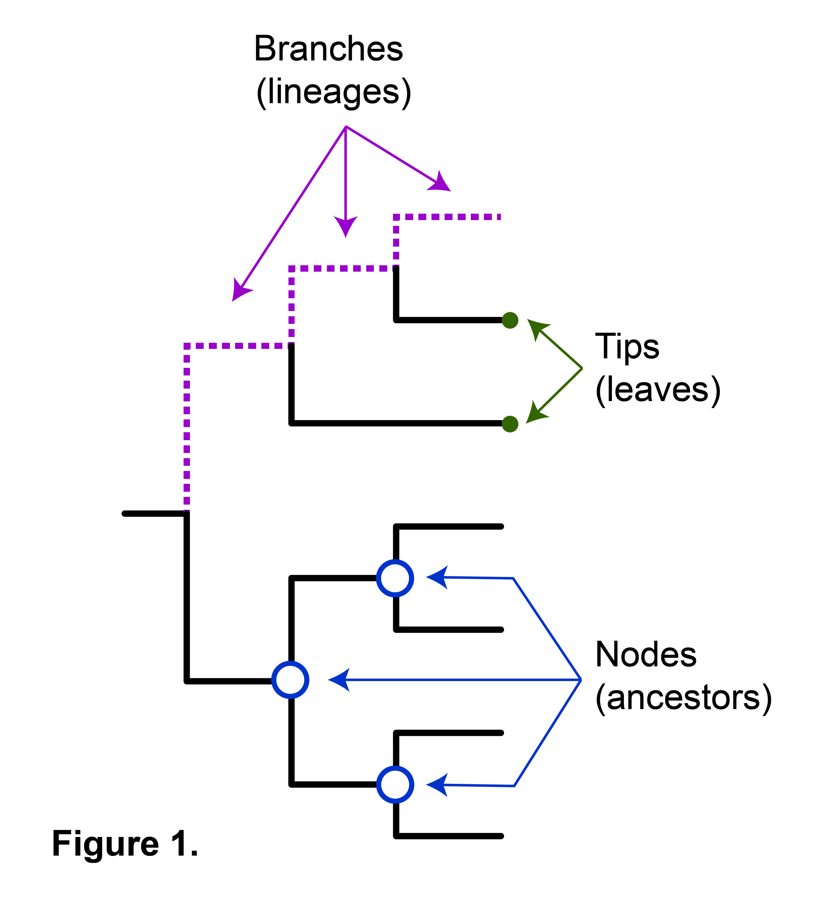
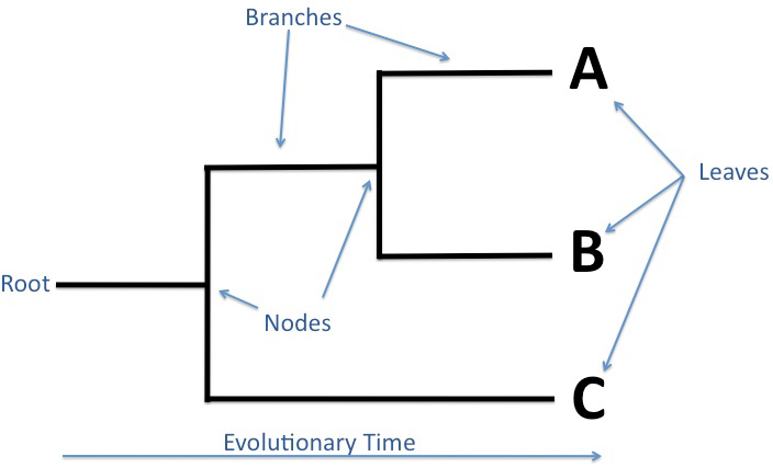
• Edge lengths in some trees represent estimated time passage.
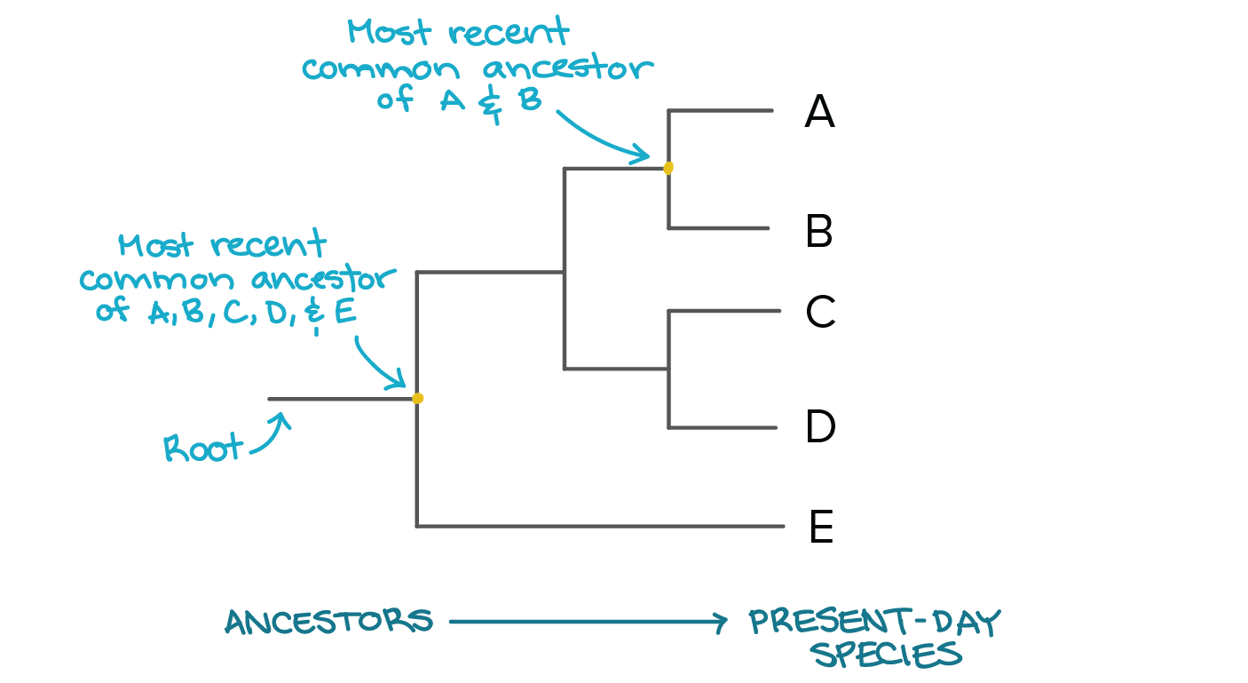
• Nodes represent the most recent common ancestor in rooted trees.
• Taxonomic units are assigned to each node.
• Internal nodes are often called hypothetical taxonomic units due to their abstract nature.
• The ""tree of life"" metaphor originates from the ancient hierarchical ladder concept.

Figure: Anatomy of Phylogenetic Tree (Source: CityU-Bioinformatics)

2. Different types of Phylogenetic Trees

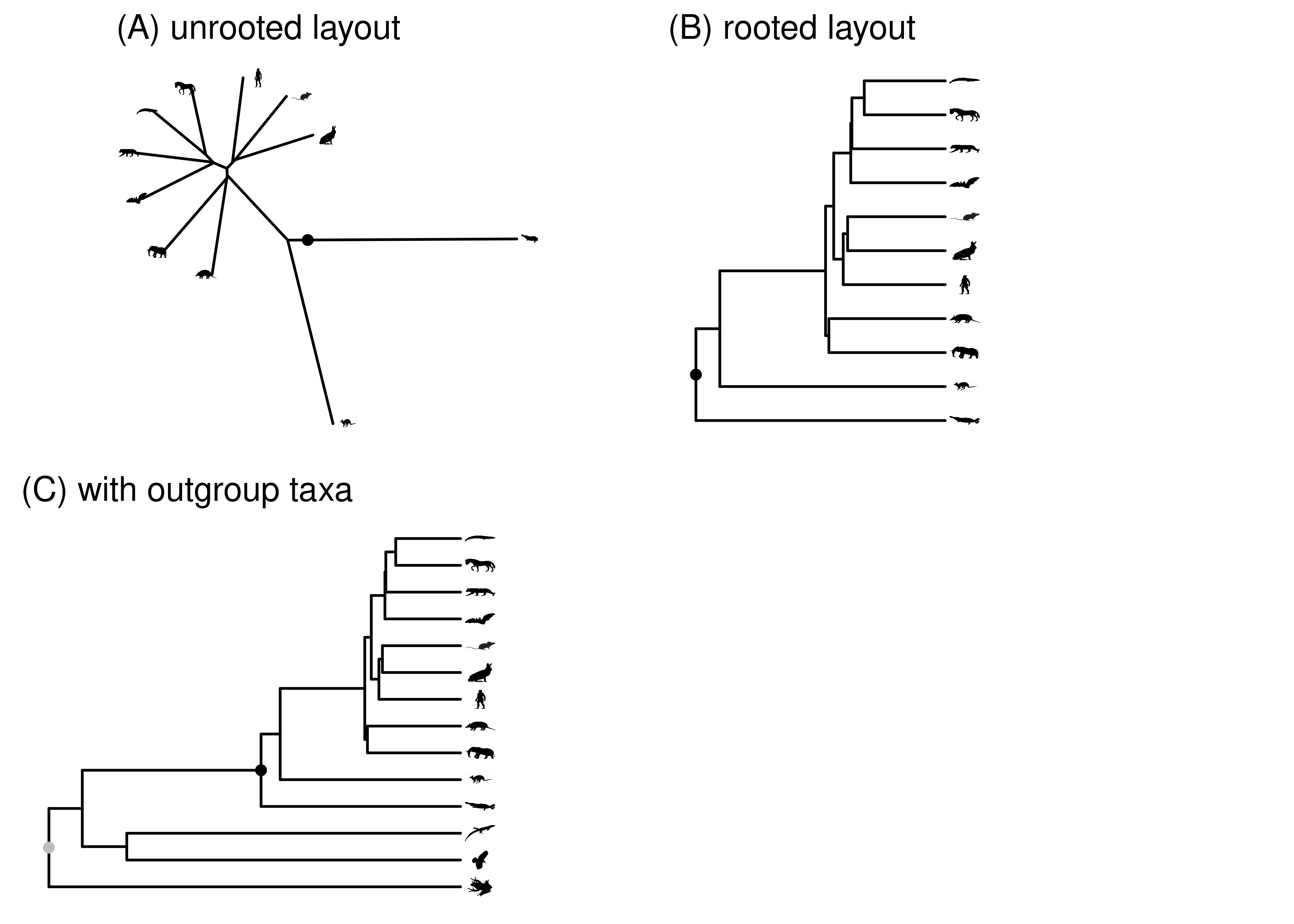
• Rooted vs. Unrooted Trees:
  • Rooted trees have a designated root node representing the most recent common ancestor. The root is the parent of all other nodes.
  • Unrooted trees don’t have a specific ancestor node. They simply show relationships between leaf nodes.
• Root Inference:
  • Rooted trees can be derived from unrooted trees by identifying an ancestor node.
  • Techniques like using an ""outgroup"" or making assumptions about evolutionary rates help determine the root.

Figure: Rooting (Source: Dunnlab)

• Bifurcating vs. Multifurcating:
  • Bifurcating trees have two branches stemming from each internal node.
  • Multifurcating trees can have more than two branches stemming from internal nodes.
• Labeled vs. Unlabeled Trees:
  • Labeled trees have values assigned to nodes (e.g., species names).
  • Unlabeled trees only show the tree structure.

3. Methods for Phylogenetic Reconstruction:

Figure: Phylogenetic Tree (Source: KhanAcademy)

3.1. Distance-based methods

Distance-based methods construct phylogenetic trees by calculating the evolutionary distances between pairs of sequences and then using these distances to infer the tree structure. Distance matrix methods use ""genetic distance"" to classify sequences, often calculated by the percentage of mismatches at aligned sites.

3.1.1 Unweighted Pair Group Method with Arithmetic Mean (UPGMA)

UPGMA is one of the simplest distance-based methods for tree construction. UPGMA (Unweighted Pair Group Method with Arithmetic Mean) is a simple and fast method that produces rooted trees and requires a constant-rate assumption. It sequentially clusters the two closest species until all are grouped.

Algorithm:

1. Calculate a distance matrix for all pairs of sequences.
2. Identify the pair of taxa with the smallest distance.
3. Join these taxa into a single cluster.
4. Recalculate distances between the new cluster and all other taxa.
5. Repeat steps 2-4 until all taxa are clustered.

Figure: UPGMA Calculation (Source: Bartleby.Com)

Strengths:

• Simple and fast
• Works well for closely related sequences

Weaknesses:

• Assumes a constant rate of evolution (molecular clock)
• Can produce incorrect topologies for distantly related sequences

Use Case:

UPGMA is often used as a quick initial analysis or for datasets where the molecular clock assumption is valid, such as in studies of closely related bacterial strains.

3.1.2 Neighbor-Joining (NJ) Method

The Neighbor-Joining method improves upon UPGMA by not assuming a constant rate of evolution. Neighbor-joining is a bottom-up clustering method that uses genetic distance as a grouping parameter. It produces unrooted trees and does not assume equal evolution rates. This method is fast but lacks accuracy due to potential bias and does not examine all possible topologies.

Figure: NJ Method (Source: Tenderisthebyte.Com)

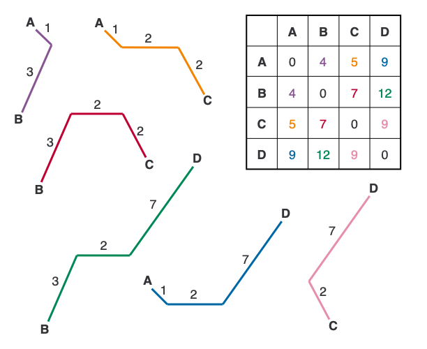
Algorithm:

1. Calculate a distance matrix for all pairs of sequences.
2. Compute the net divergence (r) for each taxon.
3. Calculate the adjusted distance (M) between each pair of taxa.
4. Find the pair with the lowest M value and join them.
5. Calculate the distance from each of the joined taxa to the node.
6. Recalculate the distance matrix for the joined taxa.
7. Repeat steps 2-6 until all taxa are joined.

Figure: NJ Method (Source: ResearchGate)

Strengths:

• Does not assume a molecular clock
• Generally more accurate than UPGMA
• Computationally efficient

Weaknesses:

• Can be less accurate for highly divergent sequences
• Sensitive to the order of input sequences

Use Case:

NJ is widely used in initial phylogenetic analyses and for large datasets where more computationally intensive methods are impractical.

3.2. Character-Based Methods

Character-based methods consider each nucleotide or amino acid position independently, treating them as discrete characters.

3.2.1 Maximum Parsimony (MP)

Maximum Parsimony seeks to find the tree that requires the fewest evolutionary changes to explain the observed data.

Algorithm:

1. Generate all possible tree topologies for the given taxa.
2. For each topology, calculate the minimum number of character changes required.
3. Select the tree(s) with the lowest number of changes.

Figure: Maximum Parsimony (MP) (Source: Slideplayer.Com)

Strengths:

• Intuitively appealing concept
• Works well for closely related sequences
• Can handle multiple character states

Weaknesses:

• Can be computationally intensive for large datasets
• Susceptible to long-branch attraction
• Assumes that character changes are rare

Use Case:

MP is often used in morphological studies or for analyzing highly conserved molecular sequences.

3.2.2 Maximum Likelihood (ML)

Maximum Likelihood estimates the tree topology and branch lengths that have the highest probability of producing the observed data under a specified model of evolution. Simulation studies show it outperforms other methods in most scenarios. It heavily relies on computers due to the vast number of possible trees. It involves a preliminary investigation of potential tree locations, sacrificing absolute certainty of finding the highest probability tree.

Figure: Maximum Likelihood (ML) (Source: DOI:10.1080/10635150117772)

Algorithm:

1. Choose an evolutionary model.
2. Generate initial tree topology.
3. Calculate the likelihood of the data given the tree and model.
4. Adjust tree parameters to improve likelihood.
5. Repeat steps 3-4 until convergence.

Strengths:

• Statistically well-founded
• Can incorporate complex models of evolution
• Generally more accurate than MP and distance methods

Weaknesses:

• Computationally intensive
• Sensitive to the choice of evolutionary model

Use Case:

ML is widely used in published phylogenetic analyses, especially for protein-coding genes and when complex evolutionary models are required.

3.3. Bayesian Inference Methods

Bayesian methods use Bayes’ theorem to calculate the posterior probability of trees given the data and a prior probability distribution.

3.3.1 Markov Chain Monte Carlo (MCMC) Bayesian Inference

MCMC Bayesian Inference samples trees from the posterior probability distribution to estimate the most probable tree and assess uncertainty. Bayesian inference uses a prior probability distribution of potential trees. This can be simple (e.g., equal probability for all possible trees) or more complex based on assumptions about evolutionary processes.

There has been debate about the use of Bayesian methods in phylogenetics due to a lack of transparency in how prior distributions, acceptance criteria, and move sets are chosen. Estimates of clade posterior probability can be inaccurate, especially for less probable clades.

Algorithm:

1. Choose an evolutionary model and prior distributions.
2. Generate an initial tree.
3. Propose a new tree by making small changes to the current tree.
4. Calculate the posterior probability ratio between the new and current tree.
5. Accept or reject the new tree based on the ratio.
6. Repeat steps 3-5 for many iterations.

Strengths:

• Provides measures of uncertainty for all parameters
• Can incorporate complex evolutionary models
• Allows for the integration of prior knowledge

Weaknesses:

• Computationally intensive
• Results can be sensitive to prior choices
• Convergence can be difficult to assess

Use Case:

Bayesian inference is increasingly popular in phylogenetics, especially for complex datasets or when estimates of uncertainty are crucial.

---

4. Tree Evaluation:

4.1. Bootstrap analysis

4.1. Likelihood ratio tests

4.1. Bayesian posterior probabilities

---

5. Practical Considerations in Bioinformatics

As a bioinformatics student, it’s essential to understand not just the theoretical aspects of these methods, but also their practical applications and computational considerations.

5. 1 Software Tools

Familiarize yourself with popular phylogenetic software:

• PHYLIP: A comprehensive package for phylogenetic analysis
• MEGA: User-friendly software for molecular evolutionary genetics analysis
• MrBayes: Bayesian inference of phylogeny
• RAxML: Maximum likelihood-based inference of large phylogenetic trees
• IQ-TREE: Fast and effective stochastic algorithm to infer phylogenetic trees by maximum likelihood

5. 2 Model Selection

Choosing the right evolutionary model is crucial for accurate tree inference. Learn to use model selection tools like ModelTest or jModelTest.

5. 3 Assessing Tree Reliability

Understand methods for assessing the reliability of inferred trees:

• Bootstrap analysis
• Jackknife resampling
• Posterior probabilities in Bayesian analysis

5. 4 Big Data Challenges

Be aware of the challenges posed by large-scale phylogenomic datasets:

• Computational complexity and runtime
• Memory requirements
• Parallel computing solutions

5. 5 Integration with Other Bioinformatics Analyses

Learn how phylogenetic analyses integrate with other bioinformatics tasks:

• Sequence alignment (multiple sequence alignment is a prerequisite for most phylogenetic analyses)
• Genome annotation
• Comparative genomics
• Molecular evolution studies

Conclusion

Mastering phylogenetic tree construction methods is a crucial skill for bioinformatics students. Each method has its strengths and weaknesses, and the choice of method often depends on the specific research question, dataset characteristics, and computational resources available. As you progress in your studies, practice implementing these methods, critically evaluate their results, and stay updated with new developments in the field. Remember that phylogenetic analysis is not just about generating trees, but about using these trees to answer biological questions and gain insights into evolutionary processes.